The Peculiar Powers of Polarisation – in maths and in the quantum realm

This part of the article gives a brief introduction to Quantum Key Distribution, one of the many exciting technologies that are actively being researched by the universities and organisations working as part of the UK National Quantum Technologies Programme.

Polarisation in technology

The very first example of humans using polarisation may have been with Vikings. It’s been proposed that one of their navigational tools may have been calcite crystals, also called “Icelandic spar” or “sunstones”, which have polarising properties. It is suggested they may have been able to infer the direction of the sun even on a cloudy day, in a way that is analogous with bees locating the sun’s location.

A much more modern use of polarisation is in Quantum Key Distribution (QKD) systems. Computers work on binary, and to protect the secrecy of messages being sent they generate ‘keys’. Keys are binary strings of 0s and 1s, and they can be used to encrypt the data sent by one computer, and decrypt the data at another computer. Normal computer encryption relies on mathematics to encrypt these messages. In a QKD system, two parties work together to generate a completely random key known only to those parties. This key can be used with other encryption methods to provide a secure method of communication. The generated key is completely random, and the way it is created relies on the laws of physics, and the quantum behaviour of light, to ensure that a third party cannot have observed the key without introducing detectable errors into the system.

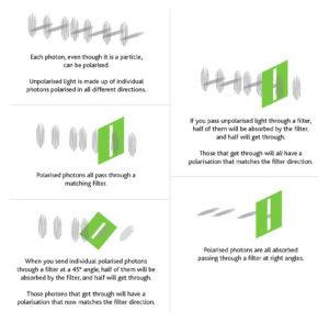
The method of QKD we are considering uses the idea that individual photons, not just waves, can be polarised.

The first party (who we call Alice) sends photons with four different types of polarisation towards the second party (Bob).

At random Alice chooses a filter direction which will be vertical or horizontal (we call these the rectilinear basis), or left-diagonal or right-diagonal (the diagonal basis) and sends a photon through it.

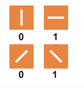
Every time Alice sends a photon that is horizontally polarised, or left-diagonal polarised, it represents a 1. At the same time vertical and right-diagonal polarisations represent a 0.

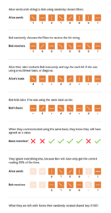
Bob also randomly chooses a filter to read the output: he will choose either horizontal or left-diagonal. Therefore, whenever Bob receives a photon, he records a value of 1. If he doesn’t receive one when he’s expecting it, then he says it’s a 0.

They then repeat this thousands of times.

Heisenberg’s Uncertainty Principle…can be stated in many ways, for different situations. In this case, if there is an eavesdropper (who we call Eve), she cannot detect the photon without altering it … and she will not know the polarisation in advance. Even when she detects it, she cannot be sure what polarisation it was transmitted with.

Even if Eve is listening in, because she doesn’t know in advance whether to use the rectilinear basis or diagonal basis, she will have to make a guess. For Eve to detect the photon she will have to absorb it. When she sends a new photon onto Bob, she will be using the same basis that she guessed with.

Half of the time she will guess correctly, and that portion of the key will be fine. Half of the time she guesses the basis incorrectly, and so will only have a 50% chance of getting the correct reading from Alice. When she sends a photon to Bob, then the reading Bob gets has only a 50% chance of being the same as Alice was sending. Therefore, whenever Eve is listening in, she will be introducing an error 25% of the time.

All Bob and Alice need to do is to compare part of their keys to make sure they agree; if there are lots of errors then they know that someone is listening in, and they know they don’t have a secure channel.

Bennett and Brassard came up with this theoretical system of generating a secure quantum key in 1984 (BB84). This, and other QKD systems, such as the entanglement of particles, are being investigated by the Quantum Communications Hub www.quantumcommshub.net.

The maths of polarisation

To understand Quantum Key Distribution, we only need to consider what happens to photons when they are arriving at 0°, 45° and 90°. However, there is a lot of interesting physics to be explored by studying light at different angles.

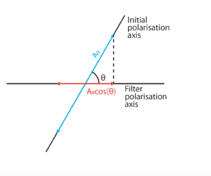
When polarised light arrives at a polarising filter at an angle, as we’ve seen, not all of it gets through. Some simple knowledge of the component of vectors can help us to determine the amplitude of the light that will get through.

A = A₀cos⁡(θ)

A = transmitted amplitude
A₀ = original amplitude
θ = the angle between the axis of polarisation and the filter

However, the intensity (energy per unit area) is not the same as the amplitude, but it is related. The intensity of a wave is proportional to the amplitude squared.

I ∝ A²

Together, this gives us the equation to determine what the intensity of transmitted light will be between a linear polarised wave and a polarised filter at an angle, θ. It is known as Malus’s Law:

I = I₀cos²(θ)
I = transmitted intensity
I₀ = original intensity

How much of the original light would get through if you used 3 filters at 30°; 90 filters at 1°; or even n filters at ${1 \over n}$°?

You can investigate multiple filters at angles using this Geogebra simulation (external website):

http://bit.ly/PolarisationModel

The future of QKD

Whilst many universities and organisations (including banking and military) are actively investigating QKD systems, there are many good engineering reasons why they are not yet seen everywhere. This is why it makes such a good topic to be studied by one of the four national hubs that make up the UK National Quantum Technologies Programme, with the eventual hope that they can miniaturise the equipment required and increase both the range and the bitrate.

The work of all four hubs is explored in more depth online using four self-study modules for students . Schools interested in this and free school-based support can register at www.stem.org.uk/quantum-ambassador-programme.

Answers

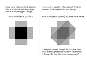
If 500 photons went through the first filter, how many of those photons do you think would make it through the final filter in this arrangement?

125 – you would lose 50% through each subsequent filter at 45°

How much of the original light would get through if you used 3 filters at 30° intervals; 90 filters at 1° intervals; or even n filters at ${1 \over n}$° intervals?

The general solution is:

$I = {I_0(cos^2 {90 \over n})^n}$

Putting the numbers in gives us for three filters:

$I = {I_0(cos^2 {90 \over 3})^3} = 0.422 = 42$%

And for 90 filters:

$I = {I_0(cos^2 {90 \over 90})^{90}} = 0.973 = 97$%